Meta-TasNet

This blog post is about the ICASSP 2020 paper Meta-Learning Extractors for Music Source Separation.¹ I will summarise and comment on the main ideas.

The goal of music source separation is to extract the signals of the individual instruments (e.g. vocals, bass, drums, guitar) from their mixture. Usually one dedicated deep neural network is trained for each target instrument separately. In this paper, the authors propose a method to separate different instruments with one single model. This is not only more parameter efficient but also allows the model to learn and exploit similarities between different instruments. The approach is inspired by meta-learning: a generator network, conditioned on instrument labels, learns to predict the parameters of a separation network, so that it separates the desired instrument. Beyond this, the paper contains some interesting ideas for source separation in the time domain.

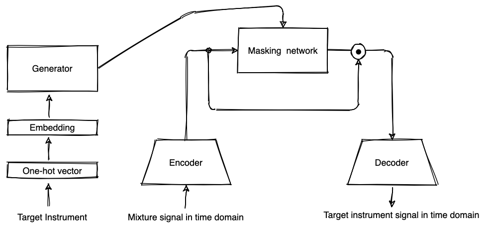
Separation network

The Conv-TasNet², which was originally proposed for speech separation, is used as a separation network. Unlike most other audio source separation models, Conv-TasNet does not rely on the short-time Fourier transform as a pre-processing step to compute magnitude spectrograms as inputs. Instead, it learns a transformation of a time domain input signal into a higher dimensional latent space with an encoder. The latent mixture representation is processed by a masking network which predicts a mask that is then element-wise multiplied with the latent mixture representation to perform the separation. The transformation of the resulting target source representation back to the time domain is done by the decoder. The authors propose some modifications to improve Conv-TasNet’s performance on music signals which I will describe in the next paragraphs.

Stronger encoder and decoder

In the original Conv-TasNet, the encoder and decoder consist of one single 1-dimensional (1-D) convolutional layer and transposed convolutional layer, respectively. Here, several 1-D convolutional layers with different kernel sizes process the mixture input. This means that a wider range of information can be captured from the wave forms. Furthermore, also a magnitude spectrogram of the mixture is computed and compressed by a linear layer. The outputs of all convolutional layers and the compressed spectrogram are concatenated and processed by two more 1-D convolutional layers to produce the latent mixture representation. The decoder mirrors the encoder to perform the inverse transformation.

It is the first time that I see someone combining the standard magnitude spectrogram with a learned representation for audio source separation. It is an interesting idea. In an ablation study, the authors show that the enhanced encoder and decoder lead to improved separation compared with the standard Conv-TasNet. However, it would have been nice to investigate also to which extent this is due to the increased capacity and due to the magnitude spectrograms as additional input.

Multi-stage architecture

The authors observed that models trained with lower sampling rates perform better on separation at 44.1 kHz. This is probably due to the limited bandwidth of the MUSDB18³ dataset which is used for training and testing. Due to compression, the songs contain barely any energy above 17 kHz. The authors propose a multi-stage architecture which first processes audio signals sampled at 8 kHz, then at 16 kHz and finally at 32 kHz. The latent target source representation of the next lower sampling rate is concatenated to the latent mixture representation of a higher sampling rate. The ablation study shows that this leads to improvements for the separation of the drums and the bass signals on MUSDB tracks. This is probably because both instruments contain a lot of low frequency content which can be efficiently encoded at low resolutions. It would be interesting to see if training at 32 kHz is also beneficial for the separation of 44.1 kHz tracks that are not compressed.

Auxiliary loss terms

Since the output is a time domain signal, the training objective for Conv-TasNet is to maximise directly the Scale-Invariant Signal-to-Noise Ratio (SI-SNR), also referred to as Scale-Invariant Signal-to-Distortion Ratio (SI-SDR)⁴. It is also used as an evaluation metric for source separation. The authors propose three additional loss terms:

• a dissimilarity loss that encourages the representations of different instruments to have little similarity
• a similarity loss that encourages the representations of the same instrument to have strong similarity across training samples
• a reconstruction loss that increases the SI-SNR of the mixture reconstruction obtained by processing the input mixture with the encoder and decoder, which are supposed to learn the transformation from the time domain to the latent space and back and should not perform any separation.

The ablation study shows that these loss terms do not improve the separation performance but the authors report that they improve training.

Generator

So far, we have focused on Conv-TasNet and the proposed extensions. However, an important part of the idea to separate different instruments with the same model is the generator. Given an instrument label as one-hot vector as an input, it predicts the parameters of the masking network so that it computes a mask to separate the desired instrument. An embedding is learned for each instrument. The parameters of each layer in the masking network are derived by two learned linear transformations of the instrument embedding.

Evaluation Results

As a baseline, the authors trained four instrument-specific versions of the (non-conditioned) Conv-TasNet with the proposed refinements. The instruments are vocals, drums, bass, and others as defined in the MUSDB18 dataset. Overall, the performance of the conditioned model, that can separate all instruments, is comparable to the one of the specialised Conv-TasNet models for the respective instruments. This reduces the required number of parameters to perform the four separations. For the instruments drums and bass the conditioned model performs better than the specialised baselines.

A comparison of the conditioned model with other recent models from the literature shows that it achieves state-of-the-art performance. However, the authors took the results of the baseline models from the respective publications. Such a comparison is problematic because different training conditions (e.g. train/validation split, data augmentation) are applied in almost every publication and influence performance. Unfortunately, the authors do not include Demucs⁵ in the comparison. Demucs is another recent time-domain music source separation model that separates different instruments at once but in a less parameter efficient way.

Conclusion

This paper presents some ideas to improve time-domain music source separation, namely, using magnitude spectrograms as additional input features, a multi-resolution architecture, and additional loss terms. Moreover, the authors showed how different instruments can be separated with one model using a control mechanism inspired by meta-learning.

It would be interesting to see if the advantage of this meta-learning approach is more evident when applied to mixtures of instruments which are more similar than the ones in the MUSDB18 set. For example, there are more similarities between instruments of a string orchestra or a choir that can be exploited. Also, the generator adds quite a lot of additional parameters to the model. A more parameter efficient approach to control music source separation with instrument labels was introduced with the Conditioned U-Net⁶. Instead of predicting model parameters, feature transformations are derived from instrument labels. Conditioning deep neural networks for audio source separation seems to be an active area of research that can lead to improved performance and efficiency.

References

---